Chapter 17 — Machine Learning with Scikit-Learn

17.0. What is machine learning?

Machine learning is a technique related to artificial intelligence and statistics. It focuses on the development of algorithms and models that enable computers to automatically learn from and make decisions about data without being explicitly programmed. In other words, it is the process of training a computer to learn patterns and make predictions based on input data. The goal of machine learning is to enable machines to improve their performance at a specific task over time as they are exposed to more data. This makes machine learning a powerful tool for a variety of applications such as natural language processing, image recognition, and recommendation systems.

Machine learning can be contrasted with what is sometimes called “Symbolic AI” or “Rule-based AI” where the behavior of the system is decided ahead of time according to a set of rules. Consider the example of making an AI for playing chess. In “Rule-based AI”, we might have a system that is programmed using explicit rules for how to behave in a situation. For example, imagine the following psuedo-code:

def choose_move():
    for game_piece in game_piece_list:
        move_list = get_move_list(game_piece)  # a function that gets the list of all the legal moves for that piece
        best_move_score = 0
        best_move = None
        for move in move_list:
            move_value = calculate_move_value(move)  # a function that returns a score for how good each move is
            if move_value > best_move_score:
                best_move = (game_piece, move)
                best_move_score = move_value
    return best_move

In that code, we might have a lot of built-in information about how good each possible move is (e.g. +10 pts for capturing a queen, +5 pts for capturing a rook, -10 pts for putting our queen in danger, etc.).

In contrast to this rule-based approach, the machine learning approach would be to let the machine figure out the best move by playing lots of games, observing the actions and consequences, and making decisions based on that. For example, a machine learning algorithm might make a move in a particular situation (i.e., with the game board in a particular state). The algorithm might keep track of what happens on the next turn, or maybe even for the next 50 turns, and “reward” or “punish” its memory of making that move in that situation based on whether there are good or bad consequences. The machine learning algorithm could, at the beginning, make random moves. But it would very quickly learn which kinds of moves lead to good outcomes and which kinds lead to bad outcomes.

Machine learning is typically divided into three different subdivisions: supervised learning, unsupervised learning, and reinforcement learning.

Supervised learning

Supervised learning is when a machine learning algorithm is given a dataset consisting of two or more variables, and trying to learn to predict the value of some variable(s) given the value of other variables. One common example of supervised learning is regression. We have already done a bit of regression, when we were trying to predict the percentage of children who say a word, given how frequent that word was in child-directed speech. Regression with just a couple of variables using simple methods is usually just called “doing statistics”, whereas when we are trying to predict values using many variables using more complex algorithms, that typically gets called “machine learning”. The boundary is blurry, debated, and not really important for our purposes.

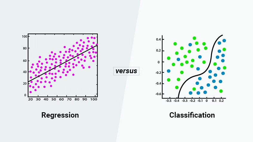
In supervised learning you will often see a distinction made between regression and classification. In regression, we are typically trying to predict a variable with quantitative values. We have already done a bit of this, when we were trying to predict what proportion of children say a word with the frequency of that word in child-directed speech. In contrast, in classification we are trying to predict binary, categorical, or qualitative values, like whether an outcome will occur or not; which of many categories some observation might belong to; or whether a photograph is one of a hot dog or not a hot dog¹. We will talk a bit about why the terms regression and classification aren’t the best terms in a later section, but it’s good to know them since you will see them used that way a lot.

The important takeaway with supervised learning is that it is called “supervised” because we know the right answer for the data we have (this value of X went with that value of Y, and this other value of X went with this other value of Y) and we are trying to use that data to develop a model (like a line or more complex curve) that models the relationship between those variables and that we can use to predict new data. Because we know the right answer for the data we have, you will sometimes see supervised learning as being used to learn relationships in “labeled” data, since we know the right “label”, or output, for every input value we have.

Unsupervised learning

Unsupervised learning contrasts with supervised learning in that we don’t have “labeled” data or right answers. We just have a bunch of variables, and are attempting to identify relationships or similarities between the data points, or to identify clusters or subgroups within the data. There are several types of unsupervised learning algorithms.

Clustering: Clustering algorithms group similar data points together based on their distance or similarity to one another.
Dimensionality reduction: Algorithms aim to reduce the number of input variables by identifying the most important features of the data. This can be useful for data visualization, as well as for reducing the computational complexity of subsequent analyses.
Association rule learning: Association rule learning algorithms identify patterns in data that occur frequently together. These algorithms are often used in market basket analysis to identify which products are frequently purchased together.

Reinforcement learning

Reinforcement Learning is like the chess example we started with. This is when an algorithm is trying to learn how to do something (like play a game), and it gets points for doing well and loses points for doing poorly. The computer learns by trying different things and seeing how many points it gets, with the goal of getting as many points as possible over time. Reinforcement learning is typically defined in terms of an agent and an environment, where the agent learns to make decisions and take actions based on feedback it receives from the environment, with the goal of maximizing its long-term reward. Reinforcement learning is commonly used in applications such as robotics, game-playing, and autonomous vehicles.

`scikit-learn`

There are many ways you can do machine learning in python. You can, of course, program algorithms from scratch, and there are times when that is what you need or want to do. But most of the time, people use modules of pre-coded algorithms for machine learning. There are many choices. You can imagine a continuum of control to these approaches, ranging from those that give you considerable control (but come at the cost of coding a lot yourself) to those that give you very little control but do almost everything for you in return. If you take a machine learning class in a CS department, you will be way over on the first side of that continuum, implimenting algorithms yourself so that you really understand them. In a more applied class, you might be over on the other end of the spectrum, where you are just trying to get a basic sense of what some of the algorithms can do. That’s what we’re going to do this week, and for that, the scikit-learn module is a good starting option. It doesn’t give you a lot of control, so in practice a lot of science and industry people don’t use it so much. But it is quick and easy to learn, and can give you a sense of what’s possible.

17.1. Two-variable linear regression

We are going to start with basic linear regression in which we try to predict a single output variable. Most people would call this “statistics” rather than “machine learning”, but it’s a good place to start. In this example, we are actually going to program everything ourselves from scratch so that we can really understand the concepts. We will then conclude by showing you the easy way to do it in scikit-learn. In future sections, we will use scikit-learn for almost everything, but we can refer to this example to understand the main concepts.

In linear regression, we have data from two variables — say,x and y — and we are trying to predict y using x. This might be trying to predict:

the number of times a rod or cone in the eye fires as a function of the brightness of a stimulus
the amount of fMRI-measured brain activity in a given brain region as a function of how surprising a stimulus is
what percentage of children say a word as a function of the number of times children hear that word
the degree of depression as a function of the amount of sleep and exercise

There are a couple basic concepts to understand about regression.

we have data that has an x and a y value, so we can view it as a scatterplot
the more these variables are predictable in terms of each other, the more easily we should be able to fit some function to the data, like a line or a curve.

Generating some correlated data

Let’s start by generating some data that makes this easy and clear to see.

import numpy as np
import matplotlib.pyplot as plt

x = np.random.normal(100, 10, 40) # an array of 40 random numbers with a mean of 100 and a standard deviation of 10
y = np.copy(x)  # make y a copy of x. we didn't just do y = x, because that would make a reference, not a copy

# add some random noise to y. For each element, we add a random value with a mean of zero, but with a stdev of
# of five. So sometimes we will add a positive, sometimes a negative, and usually a small amount.

y += np.random.normal(0, 5, 40)

plt.scatter(x, y)
plt.title("XY Scatter plot")
plt.xlabel("x")
plt.ylabel("y")
plt.show()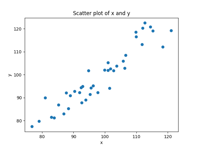

Your output if you run this code will vary slightly, of course, since the numbers are generated randomly. But what we should expect to see is a bunch of points with x values that are centered around the mean of 100, but with some pattern of distribution around that. Scores as low as 70 or as high as 130 are unlikely (about a 1% chance that any given point will be that extreme).

We know our y values will be very correlated with x; we made it that way when we started with y as a copy of x and then added some noise. If we hadn’t added the noise, every value of x and y would have been identical, and so every point would have been on a perfect line. This is what we mean when we say two variables are perfectly correlated - they lie on a line, with a positive slope for positive correlations (as x goes up, y goes up), and a negative slope as if they are negatively correlated (as x goes up, y goes down). Another way to think about variables that are perfectly correlated and on a line is that they allow us to perfectly predict one from the other. If two variables form a line, then if I know the x value, and the equation of the line, I can perfectly predict the value of y (and vice versa).

In real life, data involving anything remotely complex (like human behavior) will never be perfectly correlated. But you can end up with values that are really highly correlated, as in our example. We can actually state precisely the relationship since we generated the numbers. The value of y is likely to be the value of x, plus or minus some number that has a mean of 0 and a standard deviation of 5. That means that there is about a 66% chance that y will be within ±5 of x, and a 90% chance that it will be within ±10 of x, and a 99% chance that it will be within ±15 of x. That’s how standard deviations for normal distributions work, the standard deviation tells you the probability of values that are different distances from the mean.

Of course in real life, we don’t know the relationship ahead of time, we are trying to figure it out. So how do we do so?

Linear regression: finding the best fit line

If we don’t know the relationship ahead of time, but we think there is a linear relationship between two variables (or we want to see if there is), then what we try to do is find the line that best models the cloud of data. Look again at the figure above. You can see that you could draw a line through that cloud of points. The equation for a line is y = mx + b. But in our case, it’s really just y = x (because m = 1, and b = 0). We can add that to our scatterplot:

plt.plot(x, x, color='black')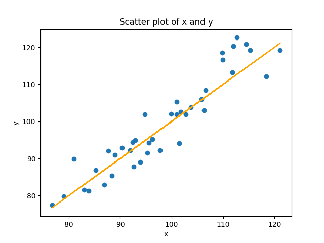

In the command above, I used x twice instead of y, so that it would plot the equation y = x. I didn’t use y because in our randomized data, y doesn’t precisely equal x because of the noise. In the real situation where we don’t know the equation, how do we figure it out?

Estimating the slope

The equation for a line is y = mx + b. m is the slope. Normally you get the slope from change in rise over change in run: (y2-y1)/(x2-x1). But we have more than two points. How do we get a line when we have more than two points? We use a method called least squares estimation, where we try to determine the line that has the shortest distance from all the points. In the case of linear equations with two variables, we can just calculate this directly.

First we multiply each value of x and y, and sum them up. When x and y are both in the same direction, each product will be positive, and when they are in different directions, each product will negative. The product will be bigger when both are big, and smaller when both are small. When we add them all up, the resulting sum will be really positive if values consistently in the same direction, really negative if they are consistently in opposite directions, and close to zero if the pattern is inconsistent, canceling out positive numbers with negative numbers.

sum_of_products = np.sum(x * y)

Next we sum all the x’s, and sum all the y’s, and then multiply these sums together. This will be bigger to the extent that all the numbers are bigger, and smaller to the extent that all the numbers are smaller. But since we aren’t multiplying each individual x by each individual y, this value doesn’t “know” anything about the relationship between x and y, just their overall size. We can use this to scale the first number, telling us if the size of the sum_of_products is big, relative to the overall size of the values.

product_of_sums = np.sum(x) * np.sum(y)

The numerator of our slope is just the sum_of_products multiplied by the number of data points, and then subtracting the product of sums. You can think of this difference score telling you “how much do x and y vary in the same direction, minus their overall size” We often call this the covariance of x and y, scaled to the number of data points n.

covariance = (n * sum_of_products) - product_of_sums

Next we need the denominator. The denominator pretty much identical, except that instead of giving us a number for the covariance of x and y, we are just looking at the variance of our predictor variable x.

x_variance = (n * np.sum(x ** 2)) - (np.sum(x) ** 2)

You can see that we are squaring each value of x and summing them up, and subtracting from the that the square of the sum of the x’s. This is the variance of x, scaled to the number of data points n. Conceptually, you can think about this by thinking about cases where the variance of x is either really high or really low. When every value of x is identical to the mean, the left and the right part will be identical. Consider a case with four scores of 3:

n * np.sum(x ** 2)
4 * (3^2 + 3^2 + 3^2 + 3^2)
4 * (9 + 9 + 9 + 9)
4 * (36)
144

np.sum(x) ** 2
(3 + 3 + 3 + 3)^2
12^2
144

At the other extreme, as the differences between the scores get higher and higher, the left side of the equation will get bigger, faster, resulting in a bigger value of the variance of x. Here’s the same simple example, but with four very different numbers.

n * np.sum(x ** 2)
4 * (5^2 + 2^2 + 4^2 + 8^2)
4 * (25 + 4 + 16 + 64)
4 * (109)
436

(np.sum(x) ** 2
(5 + 2 + 4 + 8)^2
19^2
361

Squaring numbers before you add them rises faster than squaring them after you sum them. When you square the sum of numbers, you are applying the squaring operation to the sum after it has already been calculated. This means that the contribution of each number to the sum is already equal, regardless of its magnitude. When you square the sum, the resulting value is simply a measure of the total size of the sum, without taking into account the individual values that contributed to it.

Phew. Well we now have everything we need to calculate our slope:

covariance = ((n * sum_of_xy) - (x.sum() * y.sum()))
x_variance = (n * np.sum(x ** 2)) - (np.sum(x) ** 2)
m = covariance / x_variance
print(m)

Why does that make sense as the slope? Think of it this way. The slope is a measurement of how much y changes with regard to changes in x. In our new equation, our covariance is really the same idea, how much x and y change together. The division is then just scaling that number in units of x, which is what we want, how many units does y change for each unit of x.

When I run this code on my data, I get a value of m = 1.06. Note this is really close to the “real” value of 1, but not identical. And this is because of the noise in our data. It turns out that with this data, a line with a slope of 1 is not quite the best fit to these data points, but instead a line with a slope of 1.06 is. If you run this code a hundred times, you should get values that are all centered around 1, but sometimes as low as 0.85, and sometimes as high as 1.15.

Calculating b, the y-intercept

Now how do we calculate the intercept? In the basic algebra situation, remember that once you have m, you can plug in a single (x,y) pair and get b. The problem is that we have many (x,y) pairs, and none of them are probably exactly on the line, so this approach wont work. Conceptually you can think about what we need to do is sort of figure out the “average” (x,y) coordinate and then use that with our value of m to get b. The equation below does this, though we aren’t going to walk through the explanation here (please ask if you are interested!).

b = ((y.sum() * np.sum(x ** 2)) - (x.sum() * np.sum(x * y))) / ((n * np.sum(x ** 2)) - (x.sum() ** 2))
print(b)

With this dataset, I get a value of -4.91. So again, our value is not the exact value of 0 that goes with y=x, but it is very close.

Now we can get our true line as:

print(f"The equation of the best-fit line is: y = {m:.2f}x + {b:.2f}")

output:

y = 1.06x + -4.91

The best fit line minimizes prediction error

Another way you can think about the best fit line in a model is that it is the line that minimizes the prediction error for the observed data points. Let’s look at our line again:

This is the best fit line for these points because it is the line that is the closest to each of these points. We can estimate how good of a model this is by measuring the amount of error for each point. The error for each point is just, given our model and the value of x, what value would we have predicted for y, and how did that compare to the real value of y. Add all those differences up. Well, technically add the differences after taking the absolute value, since we don’t want negative errors (predicted value is too low) and positive errors (predicted value is too high) to cancel out.

summed_absolute_error = 0  # set the error to 0

# loop through each (x,y)
for (xi, yi) in zip(x, y):
    y_predicted = b + (m * xi)  # get the predicted score for y, given that x
    summed_absolute_error += math.fabs(y_predicted - yi)  # get diff between the predicted and actual y, add to error
    plt.plot([xi, xi], [yi, y_predicted], color='orange')  # draw a line from that point to the regression line
average_error = summed_absolute_error/n  # divide the total error by n to get the average error

equation_text = f"y = {m:.2f}x + {b:.2f}"  # add the equation to our plot
error_text = f"average error={average_error:.2f}"  # add the error to our plot

plt.show()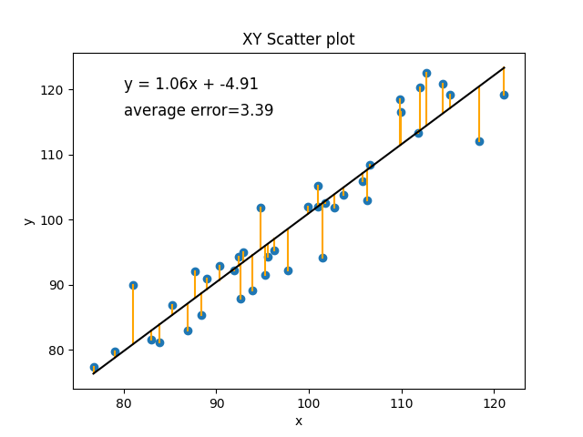

xy scatter with best fit, error lines, error text, and equation

If you imagine any other line we could draw, it would have a worse fit. Let’s just do a simple example with a different m and b that we make up to be slightly different, m=2 and b=-100.

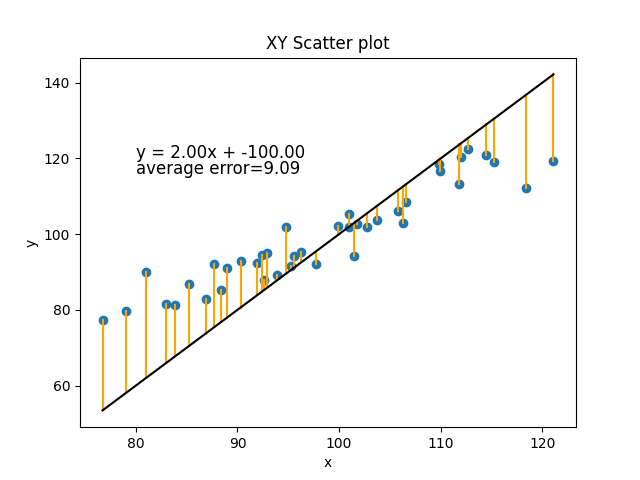
Or how about m=2 and b=0:

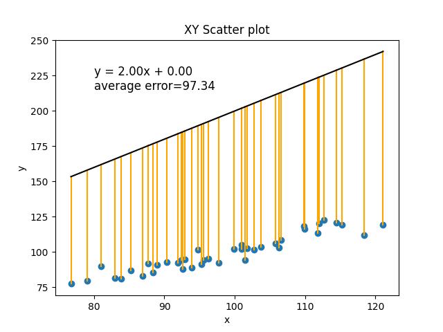
In the current situation, with the amount of random noise in our data, the best line we can make has an average error of 3.39 (every real value of y was, on average, different by about 3.39 from its predicted value).

In this section we have walked through the basic concepts of regression and how to calculate the parameters of its best fit line (m and b), and how to use that to evaluate the error of the model. We have done this the way it is typically done in statistics, by calculating those parameters directly using algebra. In the next section, we will talk briefly about why this approach doesn’t scale up to more complex kinds of functions (more variables, or nonlinear relationships), and then introduce the “machine learning” solution to that problem.

17.2. Multiple and logistic regression

In the previous section, we introduced the basic concepts of regression (predicting one variable from another), and showed how you create a linear model to do this. A linear model has two parameters (the slope m and the intercept b), which in the simple linear case can be calculated algebraically (or algorithmically using Python). Now we want to expand to show where you can take this, but why we need to change to a different approach to figuring out what the parameters of the model need to be. We’re going to talk about two main changes:

multiple (linear) regression, where we have more than one predictor variable
nonlinear regression, where we are trying to fit a curve, not just a line, to our data

Multiple (linear) regression

Multiple linear regression is the same as the linear regression we have already seen, but with more than one predictor variable. In two-variable linear regression we have the equation:

y = m*x + b

In multiple linear regression, we make the formula more general:

y = b0 + b1*x1 + b2*x2 + ... + bn*xn

As in the single predictor case, we have a single intercept. But this time we are called it b0, instead of b. This is because we are going to use b for all of our parameters. We have a different slope for each predictor, and so the slope for predictor x1 will be b1, the slope for x2 will be b2, and so on. The intercept b0 can be thought of as having its own predictor x0, which has a constant value of 1. In bigger models like this, the intercept b0 is also sometimes called the “bias” of the model, because it is biasing the value of y independently of the predictor (x) values.

Let’s again generate some data to use as a simple example. We will just use two predictor variables. So this time, instead of trying to fit a line to our 2D (x and y) data, we will be fitting a plane to our 3D data (x1, x2, and y).

This time we will specify our parameters ahead of time. We will have an intercept (b0) of 1. The slope for x1 (b1) will be -2, and the slope for x2 (b2) will be 3. Our x1 and x2 variables will again be drawn from a normal distribution with a mean of 100 for x1 and a mean of 50 for x2, both with a standard deviation of 10. We can then calculate the exact values of y given the pre-defined parameters. Now let’s also create a set of noisy_y values that add some noise to that.

n = 100
b0 = 1
b1 = -2
b2 = 3

x1 = np.random.normal(100, 10, n)
x2 = np.random.normal(50, 10, n)
y = b0 + b1*x1 + b2*x2
noisy_y = y + np.random.normal(0, 20, n)

Now let’s plot it.

# create a 3D plot
fig = plt.figure()
ax = fig.add_subplot(111, projection='3d')  # tell matplotlib this is a 3D plot

# plot the data points
ax.scatter(x1, x2, noisy_y, c='blue')

# create a meshgrid to plot the plane y = b0 + b1*x1 + b2*x2
x1_min, x1_max = np.min(x1), np.max(x1)
x2_min, x2_max = np.min(x2), np.max(x2)
x1_grid, x2_grid = np.meshgrid(np.linspace(x1_min, x1_max, 10), np.linspace(x2_min, x2_max, 10))
y_grid = b0 + b1*x1_grid + b2*x2_grid

# plot the plane
ax.plot_surface(x1_grid, x2_grid, y_grid, alpha=0.5)

# set the labels and title
ax.set_xlabel('x1')
ax.set_ylabel('x2')
ax.set_zlabel('y')
ax.set_title('3D Plane Plot')

plt.show()

Output:

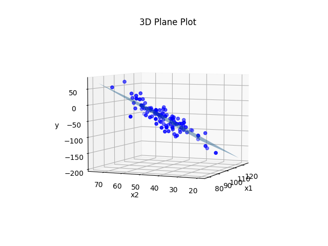
Pretty much the exact same principle as before. We plotted the plane using the real values of b0, b1, and b2 that we used to generate the data before we added noise to the y values. We could instead treat the situation like it would be in real life where we don’t actually know what b0, b1, and b2 are, and estimate those parameters from the data.

We could do it using the same procedure we did in the previous section. It’s a little more complicated because we have three variables instead of two. Instead of just needing to calculate the covariance of x and y, we need to calculate the covariance of x1 and y, x2 and y, and x1 and x2, and use all of them together. But if we did so we would end up with an equation that was something close to y = 1 -2x1 + 3x2. We could use that equation to make predicted values of y for each set of (x1,x2), and then compare those predictions to reality to get the error of the model (i.e., on average how far each point is from the plane).

The same principle can be extended out to more than two predictors. But with each variable we add, we are adding even more covariances we need to figure out. With two predictors it is three covariances: [(x1,x2), (x1,y), (x2,y)]. With three predictors it is six: [(x1,x2), (x1,x3), (x2,x3), (x1,y), (x2,y), (x3, y)]. With four predictors it is ten: [(x1,x2), (x1,x3), (x1,x4), (x2,x3), (x2,x4), (x3,x4), (x1,y), (x2,y), (x3, y), (x4, y)]. You can see that the number of covariances to estimate is starting to grow exponentially. This makes the algebraic solution to the problem start to get very computationally expensive in cases where we have many predictors. In a bit we will talk about an alternative technique.

Nonlinear regression

A second way that we can make regression more advanced is by not limiting ourselves to linear regression. Not all relationships are fit by a simple line. Many relationships are quadratic (i.e., U-shaped). Another very common nonlinear function is the one we need to use to predict qualitative outcomes. We will talk more about it in a later section, but we need to introduce it quickly here to make a point.

What happens if we want to predict a qualitative outcome, like:

will the neuron fire or not?
will a person remember a stimulus or not in a memory experiment?
is a person likely to be depressed or not?

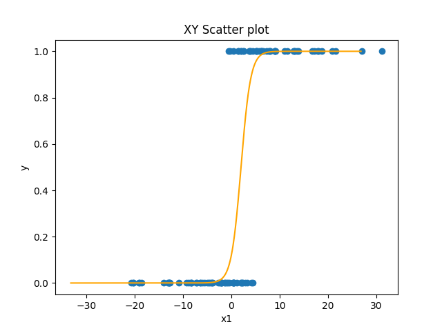
In this situation, all of our y-values are either 0 or 1. This will often result in data that looks like this: 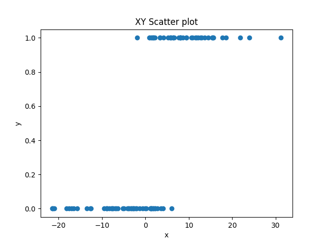binary scatter .

Here, we have a predictor variable x that varies quantitatively, and an outcome variable that varies qualitatively. As x gets bigger, y is more likely to be 1, but the relationship is not perfect. You can’t just say, “if x > 2, y=1, else, y=0”. There are some values that don’t fit this.

Sigmoid curves

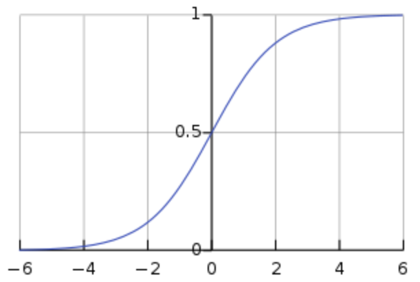
We could fit a linear regression to this data. But if you think about trying to draw a line that fit this data well, there would be a lot of points that were not on the line. An alternative is that we can fit a nonlinear function that has this shape. The most common one use in this situation is the sigmoid function:

y = 1 (1 + e^-x)

We’ll talk more about it in the next section, but the important thing for now is to see its shape:

The sigmoid function is nice because it’s x-values go from negative to positive infinity, but its y-values are limited to between 0 and 1 with a sharp nonlinear jump in the middle from one to the other. So in the simplest case (when the intercept is 0), when x is negative y is 0 or close to it. But right as x approaches zero from the negative side, y starts to go up sharply. At exactly x=0, y=0.5. And as y becomes and gets more positive, y very quickly approaches 1. The sigmoid function has the same slope and intercept parameters that a line has. As with a line, the intercept parameter shifts the curve left or right. And as with a line, the slope affects the direction and steepness of the curve.

Finding parameters for nonlinear functions

In theory, you can find parameters algebraically for nonlinear functions like the sigmoid function, the same way we did for a line. But it gets much more complicated. The nice thing about a linear function is that the relationship between a change in x and a change in y is very, well, linear. Whether you are going from x=-4 to x=-3, or x=100 to x=101, in both cases there is a change in x of 1, and so there will be an identical change in y (the slope). But in a curve, the change in y might depend greatly on the specific value of x. In the sigmoid, if the x is very negative or very positive, then a change of 1 in x might involve almost no change at all in y. Whereas if x is very close to zero, then a change of 1 in x can involve a relatively large change in y. For this reason, direct algebraic solutions become difficult, and other approaches are used.

Gradient descent optimization

An alternative to directly solve for an equation to find the slope and intercept in a line or curve is to use what is called an optimization process. An optimization process is some other algorithm that chooses a value for the parameters, and then has some algorithm by which it can nudge them in the correct direction until the right or best values of the parameters are found.

A common example of an optimization is called gradient descent learning. In gradient descent learning, we start with random values for our parameters and look at the error. It will probably be very high. Think about picking a random line to fit our linear data. Bad line. But we can actually use the information about the error for individual predictions (was the prediction too high or too low) to know what direction we need to adjust the parameters.

Consider the simple dataset below.

For each of these pairs except the last one, y = 2x + 3. The last one is close but not quite the same. So how can we use gradient descent to find that b0=3, and b1=2? We first just choose random weights. We usually want to choose random weights close to zero (assuming the values we are searching for will be distributed around zero), but not exactly zero. So maye we choose b0=1 and b1=-1. We can then go through and get predictions for each y using each x and the equation y = -1*x + 1. Then we can calculate the error of each prediction, by subtracting the real value of y from each prediction.

x   y   y_pred=-x+1    error=y_pred-y
5  13        -4              -17
2   7        -1               -8
1   5         0               -5
4  11        -3              -14
5  12        -4              -16

Intuitively we can see that our predictions were all too low, and that what we want to do is change our parameters so that we make larger predictions the next time. We can manipulate both our intercept and slope parameters to do this. But how should we change them? We can determine this algorithmically for the slope (b1) by computing the average of each x value multiplied by the error for that x. this is called the gradient for b1. We can get the gradient for our intercept (b0) by using the value of 1 (the value of x0) instead of the value of x (which is like x1, in this case). Conveniently, that is just the average of our error.

x   y   y_pred=-x+1    error=y_pred-y    b1_gradient=error*x
5  13        -4              -17           -85
2   7        -1               -8           -16
1   5         0               -5            -5
4  11        -3              -14           -56
5  12        -4              -16           -80
average x1 gradient = (-85 + -16 + -5 + -56 + -80)/5 = -37.6
average x0 gradient = (-17 + -8 + -5 + -14 + -16)/5 = -9.6

The sign (direction) of the gradient tells us the direction we want to adjust our parameters. The magnitude tells us something about how much we need to change our parameters in the specified direction. The final step is to mulitply the gradient by what is usually called the learning rate, or how big of a step in the right direction we want to take. We usually want to take small steps, for reasons we won’t go into here. So we just multiply our gradient by our learning rate (maybe a number like 0.01) and subtract that result from the parameters, to get new parameters.

theta = [1, -1]
gradient = [-9.6, -37.6]
learning_rate = 0.01
theta -= gradient * learning_rate

That’s it. That will nudge our parameters in the right direction. We can now just repeat the process over and over again, and each time the parameters we approach the right answer. Eventually, the parameters will be close to the right answer.

Here is python code that does this:

import numpy as np
import matplotlib.pyplot as plt
np.set_printoptions(precision=3)

x = np.array([5,2,1,4,5])
y = np.array([13,7,5,11,12])

# Initialize the parameters
theta = np.zeros(2)
alpha = 0.1
num_iters = 400

# Add a column of ones to the input feature for the intercept term
x = np.vstack((np.ones(len(x)), x)).T

# Perform gradient descent
for i in range(num_iters):
    # Compute the predicted values
    y_pred = np.dot(x, theta)

    # Compute the error between the predicted values and the actual values
    error = y_pred - y

    # Compute the gradient of the cost function with respect to each parameter
    gradient = np.dot(x.T, error) / len(x)

    # Update the parameters
    theta = theta - alpha * gradient

    # # Compute the cost function
    # cost = np.sum(error ** 2) / (2 * len(x))

    if i % 100 == 0:
        print(i)
        print("  x0     x1     y      ypred   error")
        print(np.column_stack((x, y, y_pred, error)))
        print("gradient:", gradient)
        print("theta:", theta)
        print()

print(f"y = {theta[0]:0.3f} + {theta[1]:0.3f}x")

Output:

x0     x1     y      ypred   error
[[  1.   5.  13.   0. -13.]
 [  1.   2.   7.   0.  -7.]
 [  1.   1.   5.   0.  -5.]
 [  1.   4.  11.   0. -11.]
 [  1.   5.  12.   0. -12.]]
gradient: [ -9.6 -37.6]
theta: [0.96 3.76]

100
  x0     x1     y      ypred   error
[[ 1.     5.    13.    12.7   -0.3  ]
 [ 1.     2.     7.     6.742 -0.258]
 [ 1.     1.     5.     4.756 -0.244]
 [ 1.     4.    11.    10.714 -0.286]
 [ 1.     5.    12.    12.7    0.7  ]]
gradient: [-0.078  0.019]
theta: [2.778 1.984]

200
  x0     x1     y      ypred   error
[[ 1.     5.    13.    12.622 -0.378]
 [ 1.     2.     7.     6.931 -0.069]
 [ 1.     1.     5.     5.034  0.034]
 [ 1.     4.    11.    10.725 -0.275]
 [ 1.     5.    12.    12.622  0.622]]
gradient: [-0.013  0.003]
theta: [3.138 1.897]

300
  x0     x1     y      ypred   error
[[ 1.     5.    13.    12.609 -0.391]
 [ 1.     2.     7.     6.963 -0.037]
 [ 1.     1.     5.     5.081  0.081]
 [ 1.     4.    11.    10.727 -0.273]
 [ 1.     5.    12.    12.609  0.609]]
gradient: [-0.002  0.001]
theta: [3.2   1.882]

y = 3.210 + 1.879x

You can see that this very quickly determines that the best slope and intercept to fit this data is a line with a slope of 1.879 and an intercept of 3.210. Let’s plot it to see:

plt.scatter(x[:,1], y)
plt.plot(x[:,1], np.dot(x, theta))
plt.xlabel('x')
plt.ylabel('y')
plt.show()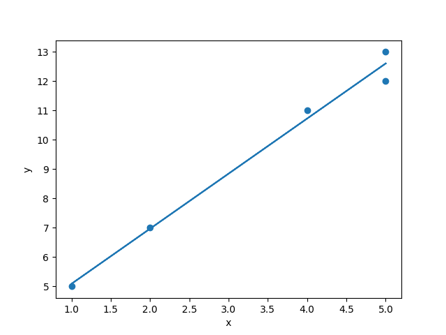

Not too shabby. Four of the observations would have fit perfectly on the line y = 3 + 2x. But because of that fifth point, we have to shift the equation a bit to y = 3.21 + 1.88x.

Gradient descent for complex regression

The gradient decent technique figured out a simple line, but we could have calculated that algebraically. Where gradient descent really shines is when you add lots of predictors, or use nonlinear functions. Remember that if we want to calculate b parameters algebraically for multiple predictors (b2, b3, b4, …, bn), we have to calculate the covariance of each pair of predictors. But with gradient descent, we only have to modify our algorithm in a very small way. All we need to do is make the x array a matrix of multiple x inputs, and modify theta so that it has a b for each x. Then we calculate the gradient for each parameter, and we can the gradient for b2, b3, or b144 exactly as we got the gradients for b0 and b1. We can then nudge them exactly the same way. So gradient descent optimization scales much better than the algebraic solution (linearly, one new computation for each new parameter, instead of exponentially).

Gradient descent is an even bigger deal for nonlinear functions. The technique works almost identically if we are trying to fit points to y = 1 / (1 + e^(-x)) as it does if we are trying to do y = mx + b. The only difference is that, in the step where we calculate the gradient, we can’t just multiply the x times the error. We need to do something more complex to handle the nonlinear relationship between x and y. But the technique is very simple and straightforward compared to the algebraic approach.

Ok, that’s it for your primer on:

how regression (predicting one variable from another) works
how to compute parameters of linear and nonlinear regression models algebraically and using gradient descent

Now let’s move on to using scikit-learn to do this quickly and easily.

17.3. Regression in `scikit-learn`

Installing `scikit-learn`

So let’s get started by installing scikit-learn. Using your terminal you can use uv to install scikit-learn:

uv add scikit-learn

Simple linear regression in `scikit-learn`

To use scikit-learn to make a linear model of this data is super easy. The only issue is that the data needs to be formatted into a matrix with columns for the different variables, and rows for the different observations. So let’s take our fake random data from the previous example, and then put it into that form.

First, let’s pick our b parameters beforehand, and generate a psuedo-random dataset using them. Remember that normally we would be using a real dataset from the real world, and we wouldn’t know these b-values. We would be trying to figure them out. But in this case we’re doing it this way to see that the regression algorithm works. Let’s do a multiple regression where we have three predictor variables (x1, x2, and x3) and an intercept x0.

Generating some pseudo-random data

import numpy as np
from sklearn.linear_model import LinearRegression


# our made-up intercept and three slopes
b0 = -1
b1 = 2
b2 = -3
b3 = 4

n = 20 # the number of observations we will generate

x = np.random.randint(-10, 10, [n, 3])  # generate a 20x3 matrix of random integers between -10 and 10
noise = np.random.randint(-5, 5, [n])  # generate a 1x20 vector of noise to add to the y value
theta = np.array[b1, b2, b3]  # create an array from our three slopes
y = noise + b0 + np.dot(x, theta)  # compute the 1x20 vector of y from y = b0 + b1*x1 + b2*x2 + b3*x3

Using sklearn to make a linear regression model

lr = LinearRegression(fit_intercept=True)
lr.fit(x, y)

And that’s it! The LinearRegression class from sklearn fits a regression model to our data, using the first argument in the .fit() function to predict the second argument. The first argument can be a matrix of any size, but the rows must be the number of observations, and the columns must be the predictor variables. The second argument must be a one dimensional array of the same size as the number of rows in the first argument. In other words, if x’s size is an m*n matrix, then y’s size must be an array of size m.

Inside the .fit() function, sklearn is running code that is pretty much exactly like what we used before. It:

assign random values to all the b’s
for num_iterations or until error < tolerance:
- for each set of x’s and y:
  - predict y using the current b’s
  - compute the error for that prediction
  - adjust the b’s to be less wrong in the future

Some options above is num_iterations and tolerance. That’s just how many times you run that loop to adjust the b’s. You can choose to do it a fixed number of times, or until the error score is below the tolerance level. For linear regression, even with many predictors, the solution is stable and guaranteed to occur, so you don’t need to worry about it too much. Whatever sklearn does automatically is fine. But with nonlinear models or more complicated algorithms we do have to worry aobut these parameters, and if we want to change them you can do so. You can read more about that here: https://scikit-learn.org/stable/modules/generated/sklearn.linear_model.LinearRegression.html#sklearn.linear_model.LinearRegression

Inspecting the model

We can examine the output in various ways. We can print the b coefficients found by the model:

print(lr.intercept_, lr.coef_)

-1.5538347833740733 [ 1.86896862 -3.01317563  4.11555825]

We can see here that we added a fair amount of noise to each y value. Without the noise, y would have been a sum of three numbers between -10 and positive 10, multiplied by 2, -3, and 4, with -1 added as the intercept. So y could have been anywhere from -91 (-1 + -10*2 + 10*-3 + -10*4) to 89 (-1 + 10*2 + -10*-3 + 10*4). We randomly added a number between -5 and 5 to each y, which is a fair amount of noise on that scale. So the resulting b parameters found by the model were not perfect. But still pretty good and close to the original real values.

We could also use sklearn to get predictions for each individual y value:

y_predict = lr.predict(x)
error = y_predict - y
for i in range(n):
    print(f"{x[i]}    {y[i]}    {y_predict[i]:0.3f}     {error[i]:0.3f}   {noise[i]:0.3f}")

As we can see in the output below, each prediction was pretty good, and the error on each prediction corresponds very closely to the noise that we added to each y value when we created them in the first place. So to the extent that there was structure in the data that could be predicted (the b-values) the linear regression found it pretty well.

x                 y    y_predict    error    noise
[9   4   6]      24     28.423      4.423   -5.000
[-7  -3  -6]    -28    -30.077     -2.077    2.000
[ 3   3  -4]    -20    -19.467      0.533    0.000
[ 0   3 -10]    -48    -48.741     -0.741    2.000
[ 8   7  -6]    -27    -28.656     -1.656    3.000
[ 1  -6   1]     22     22.432      0.432   -1.000
[-6   5  -6]    -51    -51.897     -0.897    1.000
[-1  -7 -10]    -22    -20.944      1.056    0.000
[ 2  -4  -6]    -13     -8.306      4.694   -4.000
[-5   9   9]     -5     -4.230      0.770   -3.000
[-7   8  -9]    -71    -74.456     -3.456    4.000
[-8   2  -7]    -55    -50.942      4.058   -4.000
[-3  -3   0]      1      1.284      0.284   -1.000
[-10 -5   8]     22     23.337      1.337   -4.000
[-1  -8   7]     52     47.249     -4.751    3.000
[-6   0   9]     22     20.578     -1.422   -1.000
[ 4  -2 -10]    -24    -25.451     -1.451    3.000
[ 5  -1   5]     36     31.181     -4.819    4.000
[-4  -1   4]      5      8.563      3.563   -5.000
[ 3  -4  -2]      9      9.123      0.123    0.000

We can also get the R^2 score from the model: hat percentage of the variance in the data could be predicted from the parameters:

print(lr.score(x, y))

output

0.9953803064300027

That’s a pretty good R^2 score. You’ll never get one that high on real data unless you’re studying basic physics, or you’ve screwed up your data. In the real world, data is much noisier than in our simple example.

17.4. Classification in `sklearn`

As we discussed in a previous section, we often want to predict categorical data. Which group does a particular observation belong to? There are many real world applications:

classifying emails or text messages as spam or not spam
classifying medical images as having a disease or not having a disease
classifying images, such as identifying the content of images for autonomous vehicles or recognizing faces in photos.
Object detection: In computer vision, supervised classification algorithms are used to detect objects in images and video streams.
Speech recognition: determining what word was said by a person

There are also more specific applications within Brain and Cognitive Science

Brain-computer interface: Supervised classification algorithms can be used to analyze EEG signals from the brain and control external devices like prosthetic limbs.
fMRI analysis: Supervised classification algorithms can be used to analyze fMRI data to identify brain regions that are activated during specific cognitive tasks, such as language processing, working memory, or attention.
Pattern recognition: Supervised classification algorithms can be used to identify patterns in brain activity that are associated with specific cognitive functions, such as learning, decision-making, or perception.
Diagnosis and treatment of neurological disorders: Supervised classification algorithms can be used to identify biomarkers in brain imaging data that are associated with neurological disorders such as Alzheimer’s disease, Parkinson’s disease, or schizophrenia.
Predicting cognitive performance: Supervised classification algorithms can be used to predict cognitive performance in individuals based on their brain imaging data, such as predicting working memory capacity or reaction time.

There are many algorithms you can use to do classification, and we are only going to very briefly survey a few here and show you how to use them in sklearn. But there are a couple of basic concepts to cover first. The main thing to have in mind when thinking about classification is that we have a bunch of observed data points where we know the features of those observations, and also the category to which they belong. So for example, we might have the spectrogram of a bunch of people saying the word “dog” and also a bunch of people saying “log”, and we want to learn a set of parameters that allows us to distinguish between the two, and then use those parameters to make predictions on new data.

Generating some data

As a general rule, you can think of classification as involving a feature space, and trying to learn the boundaries in that space that separate the categories. Let’s generate some data to make this clear. Sklearn has some really nice built-in functions for generating fake datasets with certain properties that can be used to test classification problems. Let’s look at the output first, and then go through the code that made them: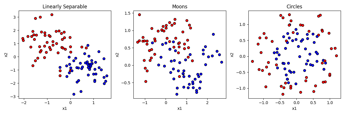

In the figure above, each of the three datasets has items that have a y value of either 0 or 1, establishing that they are either in the red or blue category. Each item also has a value for two predictor features (x1 and x2).

In the first dataset on the left, the category membership is predictable by a linear combination of x1 and x2. If an item is high on x1 and low on x2, that makes it more likely to be blue. But the relationship is not perfect. That’s like the “noise” in our earlier examples.

In the second dataset in the middle, the data is generated by a function making a little “moon” or u shape. The red items form an upside-down u on the top, and the blue items a right-side-up u on the bottom. But again the relationship is not perfect.

In the third dataset on the right, the data is generated by making two circles, with the blue one on the inside and the red one on the outside. But again the relationship is not perfect, and the circles overlap a little bit.

Here is the code that generated the data.

from sklearn import datasets

random_seed = 404  # generate all datasets with this random seed. means result will be same every time we run code

dataset_list = []  # a list for our datasets

# generates a
x, y = datasets.make_classification(n_samples=100,
                                    n_features=2,  # how many dimensions to generate
                                    n_informative=2, #  how many of the features will matter
                                    n_redundant=0, # how many of the features will be redundant
                                    n_classes=2,  # how many categories there will be
                                    class_sep=0.8, # how much the categories will overlap
                                    n_clusters_per_class=1, # if and how many subgroups there will be
                                    random_state=random_seed)

dataset_list.append((x, y))

x, y = datasets.make_moons(n_samples=100,
                           noise=0.3,  # how much the moons overlap
                           random_state=random_seed)

dataset_list.append((x, y))

x, y = datasets.make_circles(n_samples=100,
                             noise=0.2,   # how much the circles overlap
                             factor=0.5,  # the size ratio of the inner to outer circle
                             random_state=random_seed)

dataset_list.append((x, y))

And here is the code that generated the figure, if you are interested.

import matplotlib.pyplot as plt
from matplotlib.colors import ListedColormap

dataset_names = ["Linearly Separable", "Moons", "Circles"]
cm_bright = ListedColormap(["#FF0000", "#0000FF"])
fig, axes = plt.subplots(nrows=1, ncols=3, figsize=(12, 4))
for i, (x, y) in enumerate(dataset_list):
    ax = axes[i] # Select the subplot for this dataset
    ax.scatter(x[:, 0], x[:, 1], c=y, cmap=cm_bright, edgecolors="k") # Plot the points in the dataset

    # Set the title and axis labels for the subplot
    ax.set_title(f"{dataset_names[i]}")
    ax.set_xlabel("x1")
    ax.set_ylabel("x2")

plt.tight_layout()  # Adjust the layout of the subplots
plt.show()

Overfitting and cross validation

Before we go any further, we must introduce a very critical topic for machine learning, and that is the idea of overfitting. Overfitting is what happens we have an algorithm that learns parameters that perfectly match the data that you have seen, in a way that may lead the model to actually perform poorly at classifying new items because the algorithm was fitting the noise in the data, rather than just the rules that were generating the structure.

Consider our datasets again:

You can think of the classification problem as trying to draw a boundary (or set of boundaries) that gets all the red points on one side of the boundary, and all the blue points on the other side of the boundary. In the left example, we could draw a single line through the space and do a pretty good, but not perfect, job at that. A few points would be on the wrong side, accuracy would maybe be about 90-95%.

Now imagine drawing a much more complicated set of lines in the space to more perfectly get all the red on one side and all the blue on the other. If you were precise enough, you could draw a perfect boundary and classify all items with 100% accuracy. But is that what we would want?

We know that these data were generated by an algorithm that said blue = +x1 + -x2. The fact that some points don’t perfectly follow that rule is random noise. So we if have our model perfectly capture those points too, we are actually adding that noise to our model, in a way that might hurt our ability to predict new points that just follow the normal rules. Consider the blue point on middle right that is just above a red point. If we drew the boundary to get that blue point right, depending on how we did it, we may end up making a bunch of that space in the top right “blue” space. That would mean that if our model was used to classify new points up there, it would consider them blue, when in reality we know they really should be red.

Having a model fit your training data too well, in a way that is capturing noise rather than capturing signal, is what is meant by overfitting a model. How do we keep from overfitting a model? There are a couple of principles to follow.

The first principle is to not use a more complex model when a simpler one will do. This can mean don’t use more features than you need. It can also mean using a simpler model type, out of the ones we discuss below. For some problems you need a complex model. But the more complex the model, the more you are at risk of overfitting.

The second way you can guard against overfitting is by doing what is called cross validation. Cross validation is when we test our model on a dataset other than the one we trained it on, to make sure that performance is not significantly worse. If it is, there is a good chance we have overfit our model. in practice, we do not often have a second dataset. But as a partial solution what we can do is split our dataset up, train the model on part of it, and then test on the other part.

When we train models on our datasets below, we will do this by splitting up our dataset, training it, and then testing it on the remainder. On to the models!

Logistic regression

The kind of classification model, logistic regression, we have already discussed a bit. The way logistic regression works is to really think about it as a transformation of simple logistic regression into the nonlinear sigmoid shape we discussed in the earlier section. Remember the sigmoid function looks like this:

Anytime the input (x) is between negative infinity and about -4, y stays very close to zero. But at -4 it starts to rise exponentially, getting to 0.5 when x=0, and continuing to rise quickly until x=4 when it flattens out again at 1. This is nice, this means that we can have a predictor variable that varies continuously from really negative to really positive, and have that translate into saying either “yes” or “no” (1 or 0) in response to changes in that input.

So how can we use that like we did for linear regression? And what are the “parameters” like slope and intercept that can tell us about the relationship between the predictor and outcome? And what do we do if we want to have multiple predictors? The great thing about the logistic function is that it’s actually using the same linear function y = b0 + b1x1 + ... we were using before. That’s the first step is to compute the linear version, and then use that output as the input into the logistic function, like this:

z = b0 + b1*x1 + b2*x2 + ... bn*xn
y = 1 / (1 + e^(-z))

So you can think of all the different predictors (x1, x2, …) as each being a different feature giving us information about whether the item should be in the category (output=1) or not in the category(output=0). We weight each feature by its parameter, (b1, b2, …) which tells us how strongly and in what direction that gives us information about the item’s category membership, and add up all these weighted values. That’s z. Then we put z into the logistic function. If the information in z is really biased in the positive direction, we will end up with a score of 1. If the information is really biased in the negative direction, we will end up with a score of 0. If the information in z balances out and is close to 0, then we will end up with a score of 0.5 (meaning we aren’t sure if it’s in the category or not.)

So hopefully what should be clear from this explanation is that logistic regression, even though it is “nonlinear” regression, is still linear in the sense that it is determining a score (z) for each input and using that score to make a prediction. This score is a linearly weighted combination of the different input features. This means that logistic regression will generate a single line in the feature space as its decision boundary.

Let’s take a look a at how it does on our three datasets, then we will go through the code: 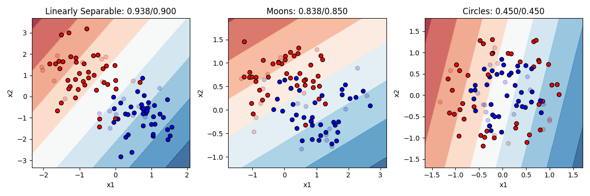Logistic Regression Results In this figure, direct your attention to a couple of things. First, notice that some points are lighter in color now. This is to visually display which point are in our training set (the darker 80% of the points) and which are in our test set (the more transparent 20%). Second, you can obviously see the background color here has been changed. This is showing the decision boundary our model is using, after it was trained on the training data. The darkness of the boundary shows where the points lie on the sigmoid curve. Right in the middle white area is where y = 0.5, the dark blue is where the model’s prediction would be 1 and the dark red where the prediction would be 0.

In our model on the left, the model is indeed pretty accurate (93% on training items and 90% on test items). We can see that it is drawing a boundary that is roughly diagonal through the space (meaning it probably has pretty equal values for b1 and b2, though one will be negative and the other positive). The single, simple linear boundary works pretty well here, since a linear boundary really was what was used to generate the data. Performance on the test items is only slightly worse.

In the other two models, the logistic regression does worse. Of course, you cannot correctly solve the circle or the moon problem with a simple line boundary. A line does ok on moons, and is actually worse than random guessing on the circles.

This demonstrates logistic regression’s strengths and weaknesses. It works very well, and is a very simple model that is unlikely to overfit the data (training and test accuracy are about the same). But it can only solve problems that are linearly separable. And unfortunatly not many problems we deal with are that simple.

Let’s look at the code. I’ve combined the code that makes the models and the figures:

from sklearn.model_selection import train_test_split
from sklearn.linear_model import LogisticRegression
from sklearn.inspection import DecisionBoundaryDisplay
import matplotlib.pyplot as plt
from matplotlib.colors import ListedColormap

dataset_names = ["Linearly Separable", "Moons", "Circles"]  # labels for our subplots
cm = plt.cm.RdBu  # the color palette for the background
cm_bright = ListedColormap(["#FF0000", "#0000FF"])  # the colors for the dots
fig, axes = plt.subplots(nrows=1, ncols=3, figsize=(12, 4))  # create the subplot figure

for i in range(len(dataset_list)):
    x = dataset_list[i][0]
    y = dataset_list[i][1]
    x_train, x_test, y_train, y_test = train_test_split(x, y, test_size=0.2)

    classifier = LogisticRegression()
    classifier.fit(x_train, y_train)

    #y_pred = lr.predict(x_test)
    train_accuracy = classifier.score(x_train, y_train)
    test_accuracy = classifier.score(x_test, y_test)

    ax = axes[i]
    DecisionBoundaryDisplay.from_estimator(classifier, x_train, cmap=cm, alpha=0.8, ax=ax, eps=0.001)
    ax.scatter(x_train[:, 0], x_train[:, 1], c=y_train, cmap=cm_bright, edgecolors="k")
    ax.scatter(x_test[:, 0], x_test[:, 1], c=y_test, alpha=0.2, cmap=cm_bright, edgecolors="k")

    # Set the title and axis labels for the subplot
    ax.set_title(f"{dataset_names[i]}: {train_accuracy:.3f}/{test_accuracy:.3f}")
    ax.set_xlabel("x1")
    ax.set_ylabel("x2")

plt.tight_layout() # Adjust the layout of the subplots
plt.show() # Display the plot

As you can see above, logistic regression is just as easy as linear regression. We have this important line:

x_train, x_test, y_train, y_test = train_test_split(x, y, test_size=0.2)

That splits our data randomly into a training set and test set with 20% of the data in the test set. Then we just create and fit the model.

This line:

DecisionBoundaryDisplay.from_estimator(lr, x_train, cmap=cm, alpha=0.8, ax=ax, eps=0.001)

is the special built in line from sklearn that draws those nice backgrounds where the boundary is. You give it your model and training set as a parameter, and it adds the color coded background to the figure.

Neural networks

A neural network is in some ways just a fancy logistic regression, but with what is called a “hidden layer”. Let’s take a look at graphical depiction of the two:

On the left is a graphical depiction of logistic regression with two predictor variables. We have parameters (b0, b1, and b2) that in the neural network context, we call weights. We compute the value of y as a function of the dot product of the input vector [x0=1, x1, x2] and our weight vector [b0, b1, b2]. The output unit (y) has what is called an activation function. If that activation function is linear, then y = dot(x, b), which is just regular linear regression. If the activation function is a ‘sigmoid’, then we have logistic regression. So a regression and neural networks with a single layer, like those on the left, are really the same thing.

But neural networks can also be made into deep neural networks with hidden layers. In this case, we have a layer of units in between the input layer and output layer. What is this hidden layer doing? Let’s think about the single layer network for a minute. In that network, the output y must be some linear combination of its inputs x1 and x2. But there is no way for it to represent a more complex function or curve. Hidden units effectively allow you to look for interactions among the inputs. So h1 could actually actually represent some complex nonlinear relationship between x1 and x2; h2 could represent a different nonlinear relationship between x1 and x2, and y could then represent a complex nonlinear relationship between h1 and h2.

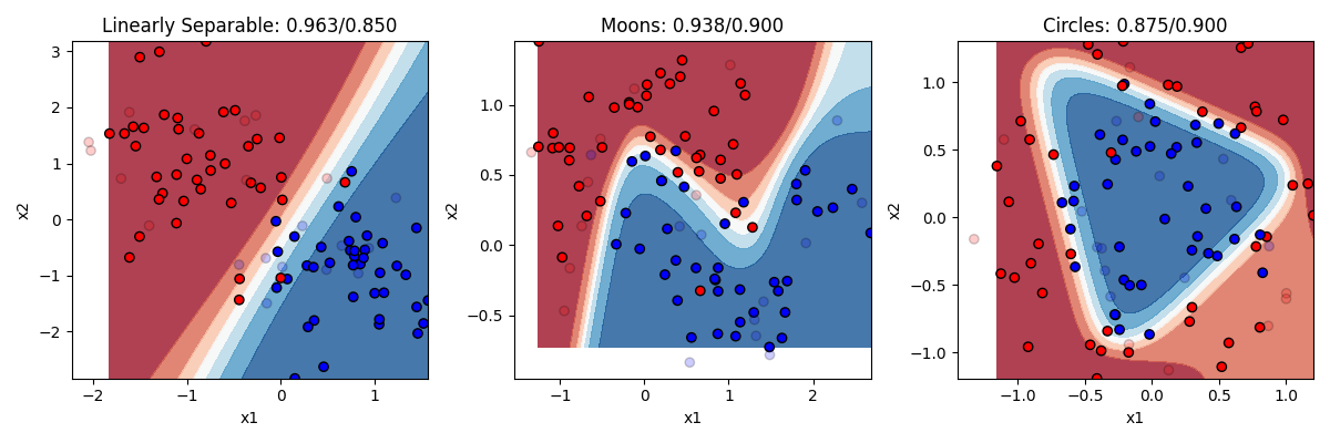
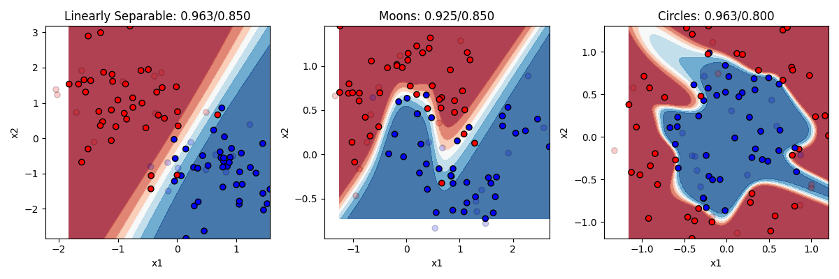
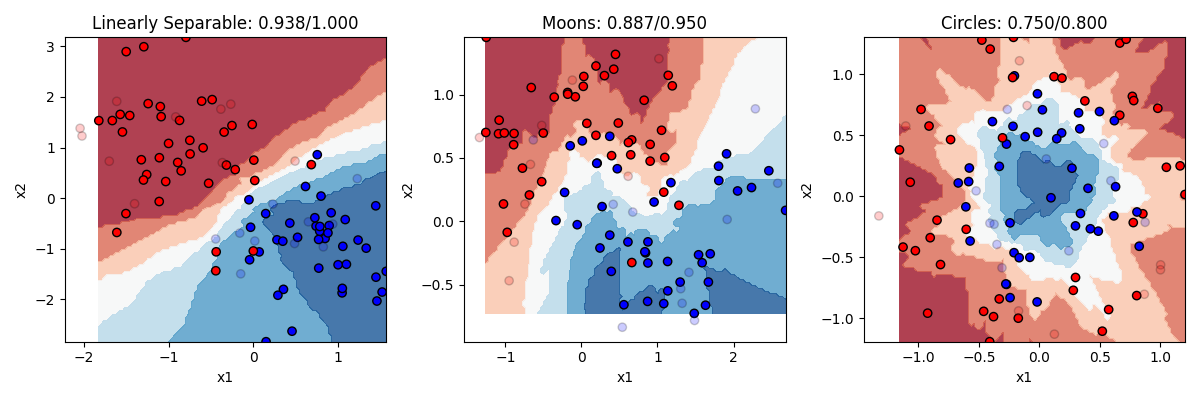
That sounds vague. What does it mean in practical terms? In practical terms remember that logistic regression was limited to drawing a single linear boundary in the space. A hidden layer allows us to draw multiple boundaries in the space. Each hidden unit allows us to draw a new line, and then y can be a function of the combination of those lines. This means we can draw a much more complex boundary through the space. Let’s see it in action. Below are three different models, one with 2 hidden units, one with 4 hidden units, and one with 32 hidden units.

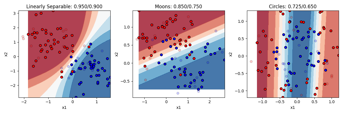
neural network with 2 hiddens neural network with 4 hiddens neural network with 32 hiddens

Remember the rule about neural networks’ hidden units: the number of hidden units is the number of lines you can draw making your boundary (with no hidden layer being 1 line). So we 2 lines at our disposal, we can end up with a curve on the linearly separable data. But remember this only needed a line, so this is actually overfitting a bit, and we can see our test accuracy drops from our training accuracy a bit. Two lines doesnt help much with the moons. Two lines helps a bit with the circles. Much better than chance now.

As we go to four hidden units we see more complex boundaries being draw in some cases. Four lines helps us draw something like a circle around the circle items, getting most of them right now. What happens when we go to 32? Overfitting on at least the problems. It is drawing a very complex boundary to capture the training items, and that leads to some big mistakes in the circle case.

The takeaway is that neural networks can allow you to solve more complex problems than simple regression, but at the cost of really raising the chance of overfitting if you don’t know how many hidden units you need to fit your data. If you work a lot with neural networks you can get better at figuring out the right number to use.

Let’s look at the code. It’s almost identical to our code before. We just need to import that model, and then change the line that created the logistic regression model to this:

from sklearn.neural_network import MLPClassifier

classifier = MLPClassifier(hidden_layer_sizes=(32),
                           activation='tanh',
                           solver='adam',
                           max_iter=5000000,
                           learning_rate_init=0.01)

Everything else stays the same. We specify our number of hidden units, our hidden unit activation function, learning parameters (solver, learning rate, and number of iterations). For some problems, you need to play around with these parameters some.

K-nearest neighbors

“K-Nearest Neighbors” (KNN) is another algorithm that is conceptually very simple. It basically takes each point you are trying to classify, and looks for its k nearest neighbors (where you get to choose the value of k) and makes a decision based on them. If k is three, and 2 of the 3 nearest neighbors are blue and 1 is red, then it will guess blue. Majority rules!

Here’s the code, just import the model and change the classifier line:

from sklearn.neighbors import KNeighborsClassifier

classifier = KNeighborsClassifier(n_neighbors=3)

Let’s see how it does with 3 and with 20 nearest neighbors 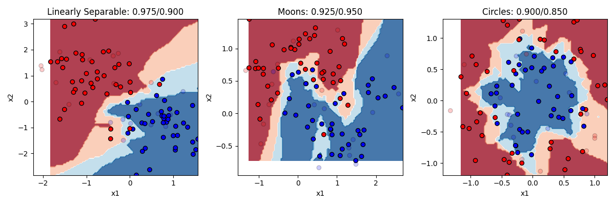neural network with k=3 neural network with k=20

KNN does pretty well. KNN is actually a really good algorithm in that it is really neutral about what is generating the data, it just looks at the neighbors instead of trying to come up with a formula to explain everything. The downside to KNN is that in order to figure out what the K nearest neighbors are, it has to calculate the distance between each point in the dataset. In our small toy dataset that’s no big deal. But if you have bigger datasets with lots of features, then it can be computationally very slow.

Decision trees and random forests

Another popular option for classification is what is called the decision tree, and its more advanced version, the random forest.

The way a decision tree works is very intuitive. The dataset is progressively divided into subsets based on individual features, with rules stating that, for that feature, what the dividing line will be. The way the decision tree makes these choices is by searching for which feature would maximize the information gain if it was split. What does this mean? Basically, it looks for a feature and a split point that would try the number of observations from a single category that could be partitioned off on one side of the split. The other side of the split would probably still have members from both categories. So then on that side of the tree another split is performed, and so on.

How many times should you split? You could keep doing this until each split contains only one category, but that might mean splitting many many times with hyperspecific splitting rules, and would probably result in overfitting. In general when people use this technique you try to split as few times as possible while maximizing your classification accuracy.

Let’s consider our linearly separable dataset. The algorithm is going to look for a feature and split point that gets as many items from one category or the other perfectly categorized. We might form a rule that says, if x2>=1.1, then guess 0, otherwise guess 1. That partitions off the whole top half of the space as ‘red’ territory. we might then form a second rule that says, if x2<1.1 and x1>0.3, guess 1, otherwise guess 0. With just these two rules we wil be oretty accurate.

Let’s look at the code.

from sklearn.tree import DecisionTreeClassifier, export_text
classifier = DecisionTreeClassifier()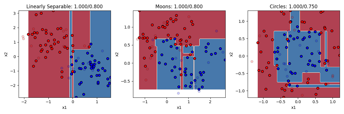

In this example we can see that the decision trees used more than two split rules (two branches of the tree). You can actually set as a parameter input how many splits to make. But you can see here that decision trees with too many splits are very prone to overfitting. They get the training dataset perfectly classified, at the cost of misclassifying too many of the test items because the rules were hyperspecific. We could change the number of splits to a smaller number to protect against this.

One nice thing about decision trees is you can print out what the decisions were that the model came up with.

r = export_text(classifier, feature_names=['x1', 'x2'], show_weights=True)

output

|--- x1 <= 0.05
|   |--- x1 <= -0.13
|   |   |--- class: 0
|   |--- x1 >  -0.13
|   |   |--- x1 <= -0.02
|   |   |   |--- class: 1
|   |   |--- x1 >  -0.02
|   |   |   |--- class: 0
|--- x1 >  0.05
|   |--- x2 <= 0.45
|   |   |--- class: 1
|   |--- x2 >  0.45
|   |   |--- x2 <= 0.76
|   |   |   |--- class: 0
|   |   |--- x2 >  0.76
|   |   |   |--- class: 1

Random Forests are an innovation on decision trees, that are designed in part to further reduce the chance of overfitting. They basically involve taking the dataset and splitting it up into many small subsets of the data, and building a decision tree for each one. Then you let each decision tree “vote” on what it thinks the right answer is for an observation, and take the winner of the vote. By sub-setting the data to a much smaller portion of the data, this makes the probability that any given decision tree might be wrong because it’s guesses will be driven by the details of which random points were in its sample. But doing it many times, the samples that have the outlier items won’t count for much, and we’ll be left with a good general depiction of the structure of the data.

from sklearn.ensemble import RandomForestClassifier
classifier = RandomForestClassifier(n_estimators=100)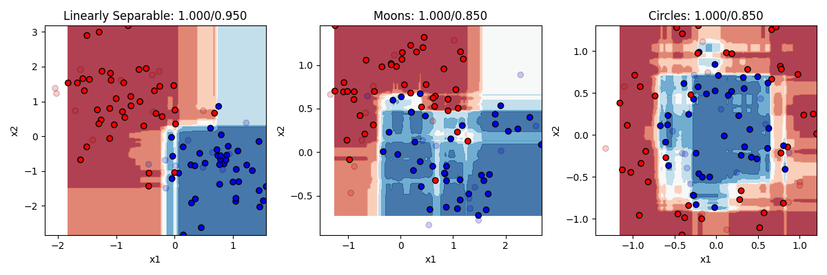

Random Forest 100 The random forest does a pretty nice job. It still overfits a little, but not too badly.

Naive Bayes

The last type of classifier to discuss is called Naive Bayes. Naive Bayes is a probabilistic machine learning algorithm that works by modeling the joint probability distribution of the input features and the target variable, and then using Bayes’ theorem to compute the posterior probability of each target class given the input features.

The “naive” assumption in Naive Bayes is that all the input features are independent given the target variable, which means that the presence or absence of one feature does not affect the probability of another feature. This assumption simplifies the calculation of the joint probability distribution and reduces the number of parameters that need to be estimated.

Here’s a step-by-step explanation of how Naive Bayes works:

Given a training dataset with input features X and target variable y, the Naive Bayes algorithm estimates the prior probability of each target class P(y) by counting the number of samples in each class and dividing by the total number of samples.
For each input feature x_i, the algorithm estimates the conditional probability of observing a particular value x_i given the target class y, denoted as P(X_i = x_i | y), by counting the number of samples in each class that have the value x_i and dividing by the total number of samples in that class.
Using Bayes’ theorem, the algorithm computes the posterior probability of each target class y given the input features X and the prior probabilities and conditional probabilities estimated in steps 1 and 2. The posterior probability is given by:

P(y | X) = (P(X | y) * P(y)) / P(X)

where P(X | y) is the joint probability of the input features given the target class, computed as the product of the conditional probabilities of each feature given the target class, and P(X) is the marginal probability of the input features, computed as the sum of the joint probabilities over all possible target classes. 4. The Naive Bayes algorithm then predicts the target class for a new input sample by selecting the class with the highest posterior probability computed in step 3.

Naive Bayes has several advantages, such as being simple, fast, and able to handle high-dimensional and sparse data. However, it may also suffer from the “zero-frequency problem” if a particular combination of input features and target class has not been observed in the training data, and from the assumption of conditional independence which may not hold in practice.

Let’s look at the code and results.

from sklearn.naive_bayes import GaussianNB
classifier = GaussianNB()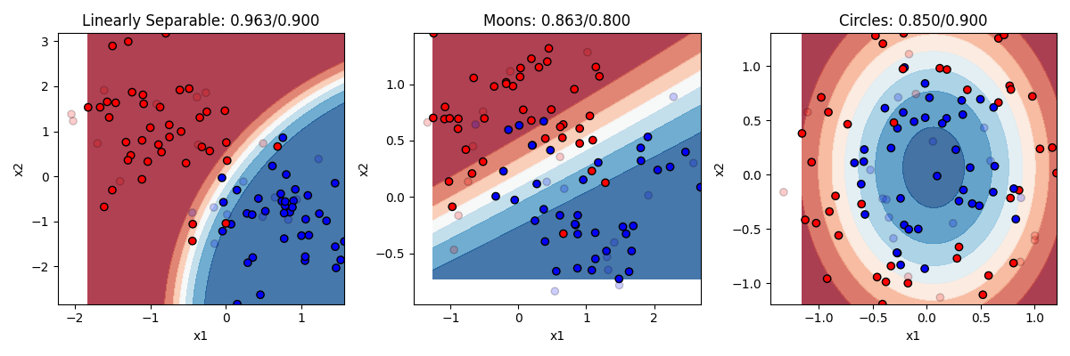

So here we can see that Naive Bayes really shines in cases where the “naive” assumption is true, and our x1 and x2 variables are independent in their effect on the probability that an observation is a y. In the “linearly separable” condition that was true, and the model gets high accuracy with little overfitting.

The assumption is also correct in the circle example on the right. Remember that the equation of an ellipse (which is what we technically have in this case) is 1 = x1^2 + x2^2. So in that equation, the effect of x1 and x2 are additive (independent), not multiplicative. Another way to say this is that there is no interaction between the two variables, i.e. the amount that x1 changes the probability that y is 0 or 1 does not affect the amount that x2 changes the probability that y is 0 or 1. In those cases Naive Bayes works very well with little overfitting. So it works pretty well for the circle case in general, and the accuracy would be quite high if not for how noisy and overlapping the two circles were.

The assumption works much less well in the moon case, where there is an interaction between x1 and x2. In order to know if a value of x1 leads y to be 0 or 1, you also need to know where you are along the x2 dimension, but in a way that isn’t a simple linear additive effect like it is for the circle. One simple way to think of this is that naive bayes can draw simple curves that additively combine dimensions, But the curve can’t have many bends in it, so it cant make the complex curve you need to predict the moons.

17.5. Clustering in sklearn

Now we are going to cover some unsupervised machine learning techniques. Remember that supervised learning is when we are trying to make a model that makes predictions about values or categories, based on labeled data where we already know the right answer or relationship between our variables. In contrast, in unsupervised learning, we are just trying to notice structure in our data to help us understand it better, but without knowing (or even trying to find) a “right answer.”

Datasets

As before, let’s start off making some toy datasets that show off the properties of our data. This time we are going to make six datasets.

blobs: some blobs that are mostly linearly separable (except for the noise)
circles: like before, circles embedded inside each other
moons: same as the last section
streaks: some streaks that are like stretched out blobs

from sklearn import cluster, datasets, mixture
from sklearn.preprocessing import StandardScaler
import numpy as np
import matplotlib.pyplot as plt
from matplotlib.colors import ListedColormap

n_samples = 200
n_classes = 4
blobs = datasets.make_blobs(n_samples=n_samples, centers=n_classes, cluster_std=2)
circles = datasets.make_circles(n_samples=n_samples, factor=0.5, noise=0.1)
moons = datasets.make_moons(n_samples=n_samples, noise=0.2)
streaks = (np.dot(blobs[0], [[0.6, -0.6], [-0.4, 0.8]]), blobs[1])
dataset_list = [blobs, circles, moons, streaks]
dataset_names = ["Blobs", "Circles", "Moons", "Streaks"]
dataset_position = [(0, 0), (0, 1), (1, 0), (1, 1)]

fig, axes = plt.subplots(nrows=2, ncols=2, figsize=(8, 8))
palette = ["#FF0000", "#0000FF", "#00FF00", "#000000"]

for i, (dataset, name, position) in enumerate(
    zip(dataset_list, dataset_names, dataset_position)
):
    ax = axes[position]
    x = dataset[0]
    y = dataset[1]
    cm_bright = ListedColormap(palette[:n_classes])
    ax.scatter(x[:, 0], x[:, 1], c=y, cmap=cm_bright, edgecolors="k")
    ax.set_title(name)
    ax.set_xlabel("x1")
    ax.set_ylabel("x2")

plt.tight_layout()
plt.show()

Output:

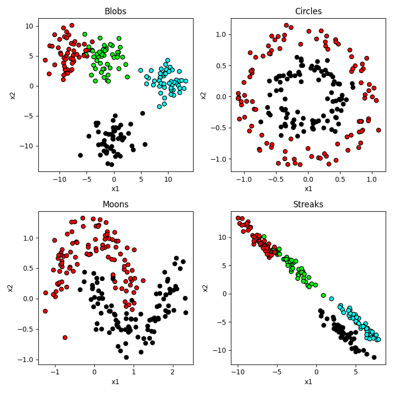
So you can see that our circles and moons have two categories used to generate the data. Our blobs are in four distinct-looking groups, although the red and green ones overlap slightly. The ‘streaks’ dataset takes those blobs and smears them out in a diagonal direction. Conceptually these groups look just as distinct, but as you will see this creates a problem for some algorithms and not others.

But of course, the whole point in this “unsupervised” section is that we don’t know any of the right answers, we are just inspecting the data to see what clusters we can find. So in our current situation, the data actually looks like this:

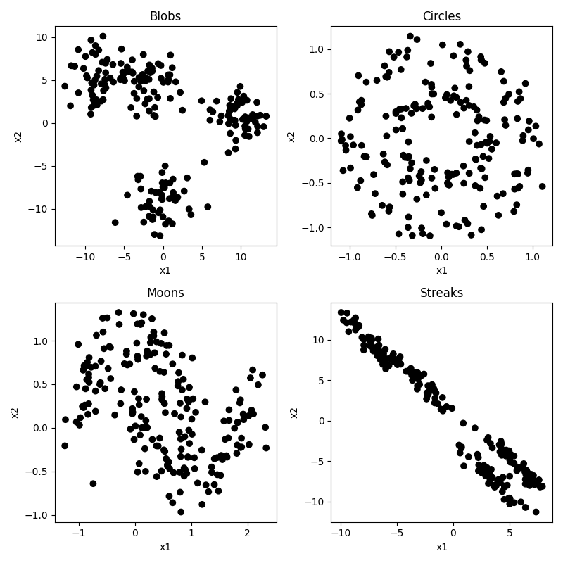
Not so easy to tell all those clusters apart now. Certainly the blobs and streaks look like two groups, not three. You can really see how having those color codes made those green and red blobs look distinct, but in reality not so much. That’s confirmation bias at work. It’s hard to look at the circles and moons without still seeing them. But how much of that is because you know they are circles and moons? We will see that some clustering algorithms have real difficulty with these categories.

Use cases for unsupervised clustering

There are many common use cases for unsupervised clustering.

The first is observation segmentation: Unsupervised clustering can be used to group observations with similar behaviors, features, preferences, or demographics together. In brain and cognitive science we might use this to group together participants, stimuli, brain regions, or behavioral responses that tend to go together in some way. In the business world, this might be used to group customers with similar behaviors, preferences, or demographics together for targeted marketing, personalized recommendations, or better customer service. For example, a company may use clustering to identify different types of shoppers based on their purchasing history, website activity, or social media interactions.

A second use case is image and text categorization. Unsupervised clustering can be used to group similar images or documents together based on their visual or textual features, for tasks such as image retrieval, content recommendation, or topic modeling. For example, a search engine may use clustering to group images of animals or landscapes together, or a news website may use clustering to group articles on similar topics. This can be used for targeted marketing, personalized recommendations, or better customer service. For example, a company may use clustering to identify different types of shoppers based on their purchasing history, website activity, or social media interactions.

A third use case is anomaly detection. Unsupervised clustering can be used to identify unusual or anomalous objects that deviate from the normal patterns or distributions of the data. This can be useful for detecting unusual behaviors in an experiment, or brain regions that are behaving very differently from other regions. In the business world, this can be used to detect fraud, intrusion, or other security breaches in financial, network, or medical systems. For example, a credit card company may use clustering to identify unusual spending patterns or locations that may indicate fraudulent activity.

A fourth use case is feature engineering. Unsupervised clustering can be used to identify important or relevant features or dimensions of the data that can be used for further analysis or modeling. This can be useful for reducing the dimensionality of high-dimensional data, identifying subgroups or patterns in the data, or generating new features or representations of the data. For example, a biologist may use clustering to identify genes or proteins that are co-expressed or co-regulated together in a particular tissue or condition.

There are many clustering algorithms. As with classification, they have their pros and cons depending on the structure of the data you are working with. Let’s take a look at some popular ones. But first we need to do one more thing.

Normalizing the data

A common first step before doing machine learning analyses is to normalize the data. This means that you are putting each predictor feature dimension on the same scale. Some dimensions may be higher variance than others, and that might mean those dimensions are getting more weight. What we do is first z-score each dimension (subracting the mean of each from each x value, and then dividing by the standard deviation). To do this we need to import the StandardScalar function form sklearn, and then call that function on our x data before we plot it or use it in a clustering algorithm.

from sklearn.preprocessing import StandardScaler
x = StandardScaler().fit_transform(x)

It doesn’t make too much of a difference in our case because our data was generated randomly with equal standard deviations used for each feature or cluster. But in a real world setting this step is critical. But you can see that the scale of our axes have changed, now going from -2 to 2 with a center at 0. We are now looking at each observation’s x1 and x2 score relative to the mean, and scaled by the standard deviation (i.e. a score of +2 means that x value was 2 standard deviations higher than the mean). And if you look really closely you can find other differences. In our original dataset, the range of the x1 and x2 axes were not always quite identical, whereas after normalization this gets evened out a bit, making each dimension count more equally.

K-means clustering

K-means is a conceptually very simple algorithm. You specify ahead of time how many groups or centers (K) you are looking for. It then tries to place those K points at places that minimizes the total distance of each observation to at least one of the K means, and then uses the closest mean to choose each observation’s cluster. Let’s see how it does. Of course, before we can do that, we would need to specify our number of clusters ahead of time. We’ll look at 2, 3, and 4.

fig, axes = plt.subplots(nrows=2, ncols=2, figsize=(8, 8))

for i, (dataset, name, position) in enumerate(
    zip(dataset_list, dataset_names, dataset_position)
):
    ax = axes[position]
    x = dataset[0]
    y = dataset[1]
    x = StandardScaler().fit_transform(x)  # normalize the data

    # run the clustering algorithm
    clustering_alg = cluster.MiniBatchKMeans(n_clusters=n_classes, n_init="auto")
    clustering_alg.fit(x)

    # get the predicted labels for each observation
    y_pred = clustering_alg.labels_.astype(int)

    # plot predicted clusters
    cm_bright = ListedColormap(palette[:n_classes])
    ax.scatter(x[:, 0], x[:, 1], c=y_pred, cmap=cm_bright, edgecolors="k")
    ax.set_title(f"{name} (MiniBatchKMeans)")
    ax.set_xlabel("x1")
    ax.set_ylabel("x2")

plt.tight_layout()
plt.show()

Here is the result for 2 Clusters. Sensible guesses, but we can see it is making some mistakes compared to the process that generated the data. The two that actually have two groups (moons, circles) are not very accurate.

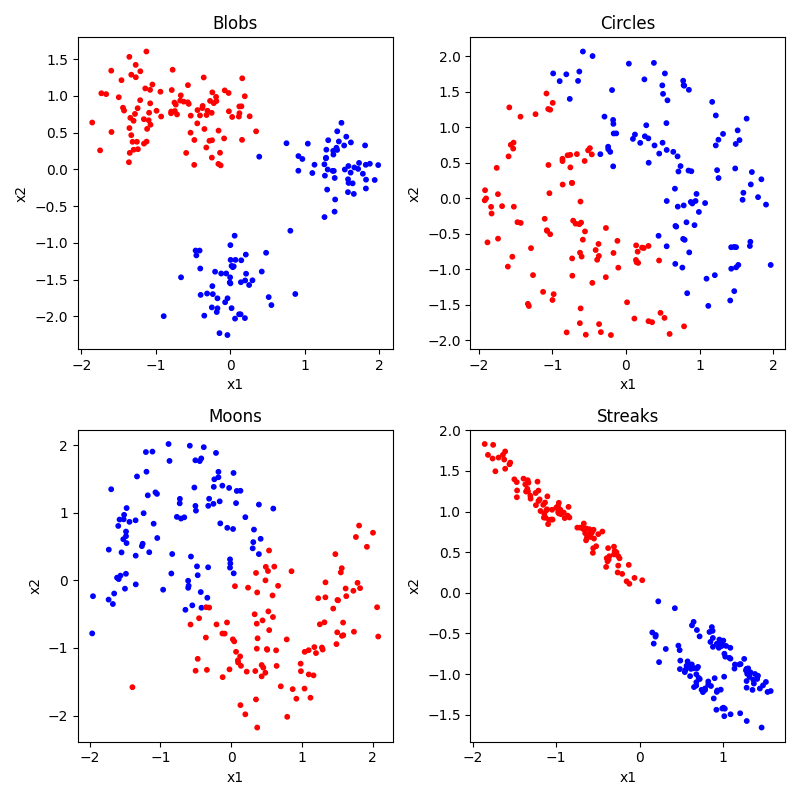
Here is the result for 3 Clusters. Bad as we would expect for moons and circles. The results for blobs and streaks are interesting. In both cases in groups two of the clusters together, but differently. In the blobs case, it can’t distinguish the two in the top left. In the streaks case it kind of separates those (though not perfectly) and groups the two in the bottom right.

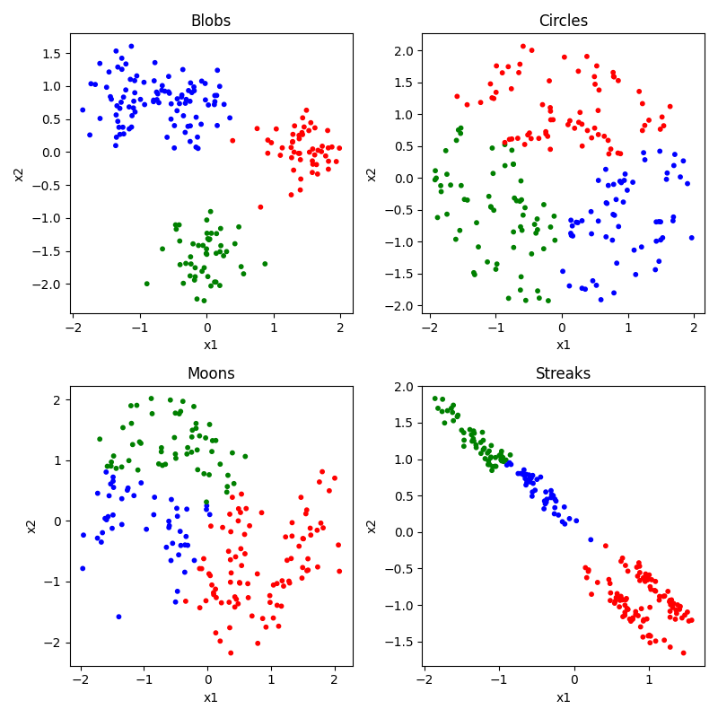
Here is the result for 4 Clusters. Again bad for moons and circles. Gets the blobs mostly right, but still really messes up the streaks. Because the streaks create so much variance along the streak from top left to bottom right, the difference between the two streaks is actually less than the difference within each streak, so it creates means that split them up incorrectly.

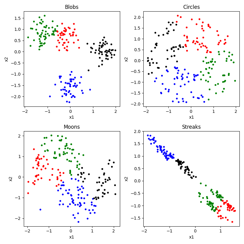
To summarize, K-means clustering is a widely used unsupervised learning technique for clustering data into groups. It has several advantages and disadvantages:

Advantages:

K-means is relatively easy to understand and implement, and it can be applied to a wide range of data types and structures.
It is computationally efficient and can handle large datasets with many variables and observations.
K-means is a simple and robust method that can handle noisy or incomplete data, and it can be used to preprocess data for further analysis or visualization.
K-means provides a natural and interpretable way to divide data into clusters based on the similarity of the data points, and it can be used for data exploration, pattern recognition, and prediction.

Disadvantages:

K-means requires the user to specify the number of clusters, which can be challenging or subjective in practice.
The clustering results can be sensitive to the initial conditions (how it randomly selects its trial mean points) and the choice of distance metric, and the algorithm may converge to a suboptimal solution.
K-means assumes that the clusters are spherical and have equal variance, which may not be true for all datasets.
K-means may not work well for datasets with overlapping or irregularly shaped clusters, or for datasets with widely varying densities or scales.
K-means does not handle categorical or ordinal data well, and it may produce different results for different data scales or normalization methods.

Despite its limitations, K-means is a widely used and effective clustering technique that can be useful in many applications. It is often used as a baseline or benchmark method for comparing other clustering algorithms, and it can be extended or modified to overcome some of its limitations.

DBSCAN clustering

DBSCAN (Density-Based Spatial Clustering of Applications with Noise) is a popular clustering method that groups data points based on their local density. In other words, it notices places were a lot of points are near each other but then separated by empty spaces, and calls those clusters. One nice thing about DBSCAN is that it doesn’t need to be told the number of clusters, it figures it out from the data.

To use DBSCAN, just swap out the model lines in the code above:

clustering_alg = cluster.DBSCAN(eps=0.3)

Output: 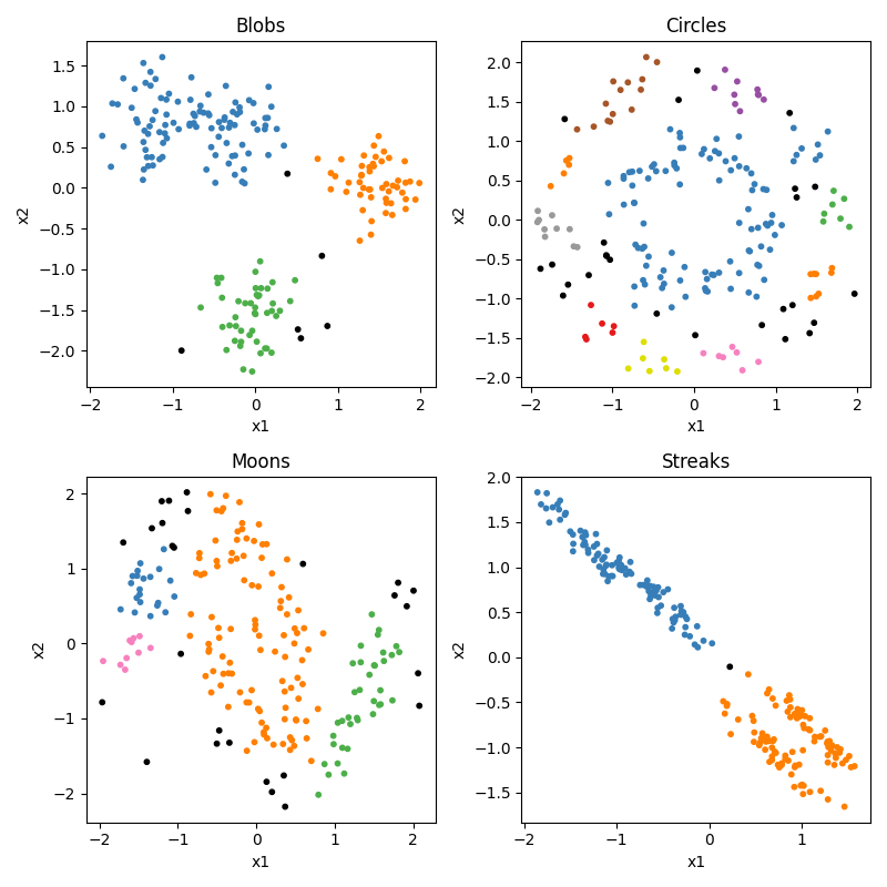DBSCAN Clustering

So we can see that DBSCAN appears to do ok, but not great. But the trick with DBSCAN is that it really relies on that eps parameter. What is eps? Eps is how sensitive the algorithm is being to the density, i.e., how close does it require points to be to group them together. At its maximum (1.0) it doesnt care how big the relative gap is, it just groups everything together into one big group. At its minimum, it treats every point as a different cluster. So with many datasets you can get good or bad performance with different settings, depending on the relative density of the clusters.

Advantages:

DBSCAN can handle datasets with arbitrary shapes and sizes of clusters, and it does not require the user to specify the number of clusters beforehand.
DBSCAN can identify noise points, which do not belong to any cluster, and it can handle outliers effectively.
DBSCAN is computationally efficient and can handle large datasets with many variables and observations.
DBSCAN is a robust method that is less sensitive to the initial conditions and the choice of distance metric compared to other clustering methods.
DBSCAN can be used for a wide range of data types and structures, including non-numerical data and mixed-type data.

Disadvantages:

DBSCAN requires tuning of the two parameters: epsilon (the radius of the neighborhood around each point) and minPts (the minimum number of points in the neighborhood required to form a dense region). Choosing these parameters can be challenging, especially for high-dimensional or sparse data.
DBSCAN can have difficulty handling datasets with varying density or with clusters of different sizes and densities.
DBSCAN may not be able to find clusters in datasets with low-density regions or with noise that is spread throughout the data.
DBSCAN can be sensitive to the choice of distance metric and may require data preprocessing or normalization.

Spectral clustering

Spectral clustering is a clustering method that takes the original x matrix and performs singular value decomposition (SVD) on it. This is basically a way to reduce the dimensionality of the data, and or to replot the data in way that better organizes the variance in the dataset.

In our 2D dataset, imagine that could redraw the two axes in any orientation, with the stipulation that they must stay perpendicular. You can, in addition, then stretch or squeeze the data along the new dimensions. Take our streak data and imagine drawing a diagonal axis that divided the top left from the bottom right, and then a perpendicular axis that divided the top right from the bottom left. But then also imagine that you could pull on the top right corner and the bottom left corner, stretch out the data along that axis. That would make some streaks pull away from each other and be less likely to be grouped together.

How it works:

Construct a similarity matrix that measures the similarity between each pair of data points. This can be done using a distance metric such as Euclidean distance or a kernel function such as Gaussian kernel.
Compute the eigenvalues and eigenvectors of the similarity matrix using singular value decomposition (SVD).
Project the data points onto the eigenvectors to obtain a lower-dimensional representation of the data.
Apply a clustering algorithm, such as k-means, to the lower-dimensional representation to group the data points into clusters.

So as you can see, spectral clustering is actually something you do in addition to one of the other approaches. So let’s try it with kmeans. Here’s the code to do it with four clusters:

clustering_alg = cluster.SpectralClustering(n_clusters=4,
                                            eigen_solver="arpack",
                                            affinity="nearest_neighbors",)

Output:

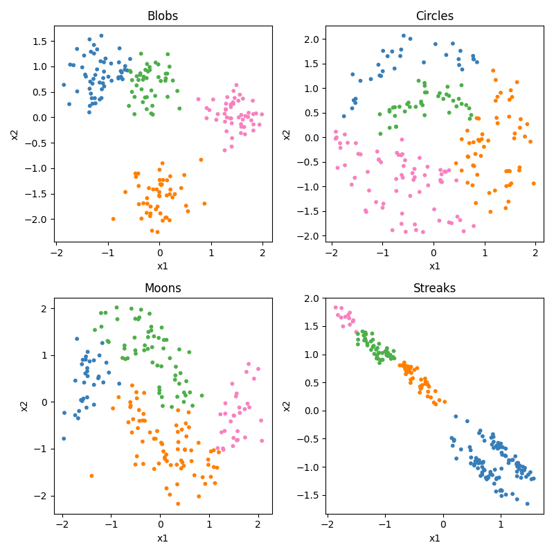
So it does the blobs well, but kmeans alone did too. It’s still not good at the circles. It does do something interesting with the moons. It doesn’t get them right, but it gets them half right. Each half moon is in a different category. Here is where the clustering could be useful, it could help you see that there are moons there once it shows them to you spit in half.

Advantages:

Spectral clustering can handle datasets with non-linear or non-convex shapes and can capture complex structures in the data.
Spectral clustering can handle datasets with varying density or with clusters of different sizes and densities.
Spectral clustering can handle high-dimensional data and can reduce the dimensionality of the data to improve the clustering performance.
Spectral clustering is less sensitive to the initial conditions and the choice of distance metric compared to other clustering methods.
Spectral clustering can be used for a wide range of data types and structures, including non-numerical data and mixed-type data.

Disadvantages:

Spectral clustering requires the user to choose the number of clusters, which can be challenging or subjective in practice.
Spectral clustering can be computationally expensive and memory-intensive, especially for large datasets.
Spectral clustering can be sensitive to the choice of distance metric, kernel function, or other hyperparameters.
Spectral clustering may not be able to handle noisy or outlier data points effectively, and it may require data preprocessing or normalization.

Despite its limitations, spectral clustering is a popular and effective clustering method that can be useful in many applications. It is often used as a baseline or benchmark method for comparing other clustering algorithms, and it can be extended or modified to overcome some of its limitations.

Hierarchical clustering

The last approach we want to show you is a bit different. It’s called hierarchical clustering.

Hierarchical clustering is a clustering algorithm that groups similar data points into nested clusters by recursively merging or splitting clusters. It creates a hierarchy of clusters that can be visualized as a tree-like diagram, called a dendrogram. Hierarchical clustering can be either agglomerative, where each data point starts in its own cluster and pairs of clusters are merged in a bottom-up fashion, or divisive, where all data points start in one cluster and clusters are recursively split in a top-down fashion.

Here is the code. We are going to generate a different dataset here, just with the blobs, to make a point about how it works:

from sklearn.datasets import make_blobs
from scipy.cluster.hierarchy import dendrogram, linkage
import matplotlib.pyplot as plt

# Generate example dataset
# the centers is what allows us to create blobs that have have sub-clusters within the blobs.
# the numbers specify where the blob centers should be.
centers = [(.5, 2), (-.5, -2), (.5, -2), (-.5, 2)]
X, y = make_blobs(n_samples=200, centers=centers, cluster_std=1, n_features=2)

# Perform hierarchical clustering
Z = linkage(X, method='ward')

# Create figure with two subplots
fig, (ax1, ax2) = plt.subplots(1, 2, figsize=(10, 5))

# Plot scatter plot on the left subplot
colors = ['red', 'blue', 'green', 'purple']
for i, center in enumerate(centers):
    X_center = X[y == i]
    ax1.scatter(X_center[:, 0], X_center[:, 1], c=colors[i], label=f'Center {i+1}')
ax1.legend()
ax1.set_title('Scatter Plot')
ax1.set_xlabel('Feature 1')
ax1.set_ylabel('Feature 2')

# Plot dendrogram on the right subplot
dendrogram(Z, ax=ax2)
ax2.set_title('Hierarchical Clustering Dendrogram')
ax2.set_xlabel('Index')
ax2.set_ylabel('Distance')

plt.tight_layout()
plt.show()

Output: 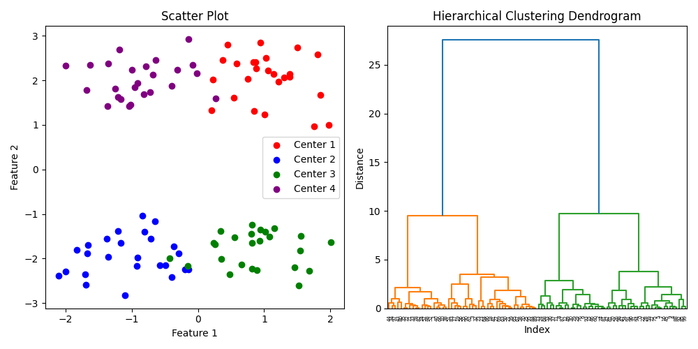Scatterplot and HC Dendogram

Overall, hierarchical clustering is a powerful tool for clustering analysis that provides a flexible and interpretable approach to grouping similar data points. However, its computational complexity and sensitivity to noise and outliers can be limitations in certain applications.

Advantages

Flexibility: Hierarchical clustering can be used with different distance metrics and linkage criteria, allowing it to handle a wide range of data types and structures.
Interpretability: The dendrogram generated by hierarchical clustering provides a visual representation of the hierarchical structure of the clusters, which can be used to interpret the relationships between the data points.
No assumption of the number of clusters: Hierarchical clustering does not require specifying the number of clusters in advance, which can be advantageous when the number of clusters is not known a priori.

Disadvantages

Computational complexity: The time and memory requirements of hierarchical clustering can be significant, especially for large datasets.
Lack of scalability: Hierarchical clustering may not scale well to very large datasets, or datasets with high dimensionality, due to the computational complexity of the algorithm.
Sensitivity to noise and outliers: Hierarchical clustering can be sensitive to noise and outliers, which can affect the quality of the resulting clusters.
Lack of flexibility in merging and splitting: The agglomerative and divisive nature of hierarchical clustering may not be appropriate for all data structures, and may not allow for the discovery of complex cluster structures.

17.6. Lab 17

import numpy as np

def q1():
    print("Question 1")
    '''
    The reading discussed how you can calculate parameters in a regression algebraically, and also using an
    optimization technique. Describe how they are different, and what the reading said about what the situations
    are where you would want to do it one way versus the other. Use a print statement to display your answer.
    '''


def q2():
    print("Question 2")
    '''
    According to the reading, what is the difference between supervised and unsupervised learning? According to
    the reading! I know what the top 5 google answers are, and what ChatGPT would say. The reading gives a specific
    explanation I want you to understand. Answer the question in a print statement.
    '''

def q3():
    print("Question 3")
    '''
    According to the reading, linear regression is bad for predicting certain kinds of data. What are two examples
    that were given? Answer the question in a print statement.
    '''

def q4():
    print("Question 4")
    '''
    The reading gave code and walked through how to find the slope and intercept using gradient descent
    optimization. We got this equation:
    y = 3.210 + 1.879x

    In a previous section we also showed how to calculate the parameters algebraically. Replicate that code inside
    this function, and see if it provides the same result. Print the equation you get. If it is not quite the same,
    explain in a print state why this makes sense.

    '''
    x = np.array([5, 2, 1, 4, 5])
    y = np.array([13, 7, 5, 11, 12])


def q5():
    print("Question 5")
    '''
    Take the code I provided to calculate a linear slope and intercept using gradient descent for one predictor
    variable, and modify it to work with n predictor variables. Then use it on the data below, where each column of x is
    a different predictor variable, and each row of x is a different observation. When you are done you should print
    out the regression equation y = b0 + b1x1 + b2x2 + b3x3, substituting in your four parameter values for the four b's.
    The right answer will be something like y = -4 + 2x1 - 3x2 + 4x3, but not exactly.
    '''
    x = np.array([[1, -10, -6],
                  [-3, 6, -2],
                  [7, -10, -5],
                  [-10, 1, -8],
                  [2, -6, -9],
                  [-4, -4, 7],
                  [-1, -7, 4],
                  [6, 6, 5],
                  [-9, 7, -6],
                  [-1, 8, 0],
                  [-9, -1, 0],
                  [7, -2, 2],
                  [2, -9, -4],
                  [-4, -9, -2],
                  [-2, 2, -5],
                  [-3, 1, 3],
                  [-10, 5, 8],
                  [-3, -6, -6],
                  [0, 0, 2],
                  [-6, 5, 4]])
    y = np.array([4, -36,  20, -59, -18, 28, 31, 10, -67, -30, -19, 24, 11, 7, -34, -1, -7, -16, 4, -15])

def q6():
    print("Question 6")
    """
    Load the mcdi dataset (https://github.com/stefanuddenberg/python_for_bcs/blob/master/ebook/data/lab10/predict_mcdi.csv)
    into a DataFrame. Use that data and sklearn's linear regression to
    compute a linear regression model predicting MCDIp using
    Age, LogFreq, and ProKWo as predictor variables. Print the resulting equation, and interpret it in a print statement.
    Also print and interpret the model's R^2 score.
    """

def q7():
    print("Question 7")
    '''
    In data/lab11/, there are two files:
    - concepts.csv: a file with two columns, a list of concepts, and a 1 or 0 on whether it is an animal or not
    - feature_matrix.csv: a file with values from an experiment where human subjects were asked to list the
        features or properties of a each word. Each row is a concept corresponding to the concepts in the first
        file (and in the same order). THe columns represent the different features in people listed in the
        experiment. For example, the first column is "a_musical_instrument". The value of the cell [0,0] is
        .933, representing that 93.3% of subjects listed that feature for the first concept, accordion. Cell
        [1,0] has value of 0, representing that zero subjects said "a musical Instrument" for alligator.

        You are going to try to classify whether each concept is an animal or not, using the feature vector
        for each concept. Pick two of the classifier models discussed in the reading, and use it to classify
        the entire dataset. Remember to randomly divide your dataset into a training set and a test set, using
        80% of the data in the training set, and 20% in the test set. Print which classifier you used, and
        your accuracy for each classifier.
    '''

def q8():
    print("Question 8")
    '''
    Now use the same dataset to do unsupervised clustering. Pick two of the clustering algorithms described
    in the reading.
    '''

def q9():
    print("Question 9")
    '''
    Create a clustering dendrogram for the different concepts in the feature dataset.
    '''


def main():
    q1()
    q2()
    q3()
    q4()
    q5()
    q6()
    q7()
    q8()
    q9()


if __name__ == "__main__":
    main()

See “Silicon Valley” Season 4 Episode 4 for the reference.↩︎

17.0. What is machine learning?

Supervised learning

Unsupervised learning

Reinforcement learning

scikit-learn

17.1. Two-variable linear regression

Generating some correlated data

Linear regression: finding the best fit line

Estimating the slope

Calculating b, the y-intercept

The best fit line minimizes prediction error

17.2. Multiple and logistic regression

Multiple (linear) regression

Nonlinear regression

Sigmoid curves

Finding parameters for nonlinear functions

Gradient descent optimization

Gradient descent for complex regression

17.3. Regression in scikit-learn

Installing scikit-learn

Simple linear regression in scikit-learn

Generating some pseudo-random data

Using sklearn to make a linear regression model

Inspecting the model

17.4. Classification in sklearn

Generating some data

Overfitting and cross validation

Logistic regression

Neural networks

K-nearest neighbors

Decision trees and random forests

Naive Bayes

17.5. Clustering in sklearn

Datasets

Use cases for unsupervised clustering

Normalizing the data

K-means clustering

Advantages:

Disadvantages:

DBSCAN clustering

Advantages:

Disadvantages:

Spectral clustering

Advantages:

Disadvantages:

Hierarchical clustering

Advantages

Disadvantages

17.6. Lab 17

`scikit-learn`

17.3. Regression in `scikit-learn`

Installing `scikit-learn`

Simple linear regression in `scikit-learn`

17.4. Classification in `sklearn`